Three Probability Lenses on America’s Market Outlook

How Reliable Are Century-Old Stock Market Returns?

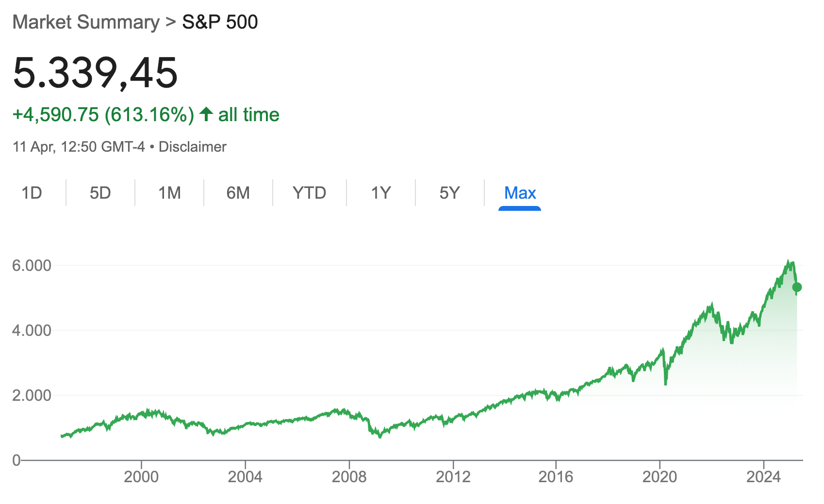
The U.S. stock market has traditionally been the global benchmark for steady growth and reliable returns—often cited as averaging about 9.8% annually over the long haul.

Yet, I find myself questioning whether this “golden track record” still holds up for the decades ahead. Are we really destined to continue enjoying those historically robust returns, or might changing world dynamics reduce that figure in ways we’ve yet to fully understand?

In this post, I’ll expand on that question by examining four key areas in depth:

1. Historical Perspective on Returns: A closer look at where that 9.8% figure comes from, how reliable it is, and how real (inflation-adjusted) returns have varied across eras.

2. Probability Theory in Markets: An exploration of probability interpretations – relative frequency, propensity, and subjective belief – and how each might frame our understanding of stock market behavior.

3. Complexity and Prediction Limits: Insights from Michael Mauboussin and others on why markets are complex adaptive systems that defy easy forecasting, the role of base rates, and common forecasting errors.

By the end of this post, I hope to offer a more nuanced perspective on how we should think about future return forecasts—one that balances historical evidence, inherent forces, and a dash of personal judgment.

Part 1: Historical Perspective on U.S. Stock Market Returns

Most discussions of long-run stock performance reference roughly 10% average annual returns for U.S. equities. For example, the S&P 500 index (including dividends) has delivered about 9.9% per year as of early 2025 over many decades​.

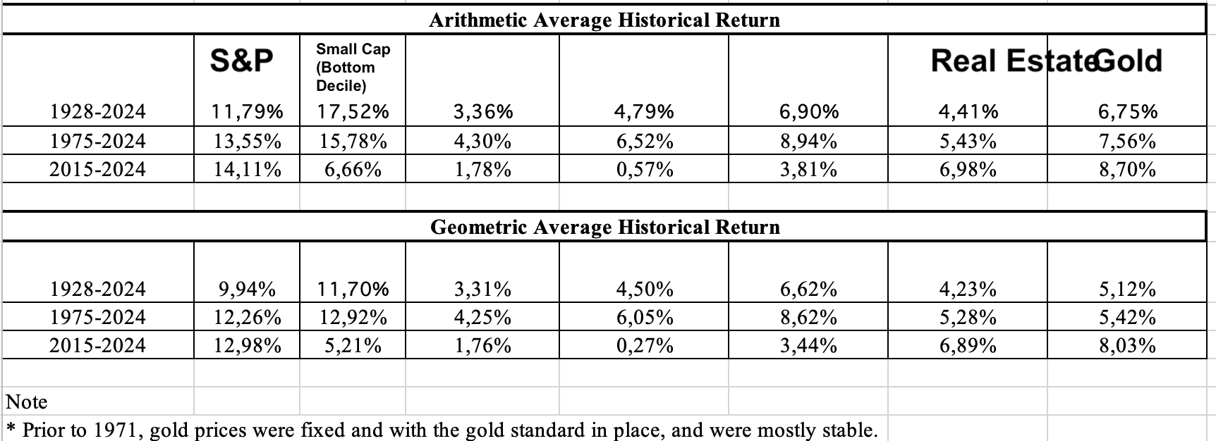
(Source: NYU: “Historical Returns on Stocks, Bonds and Bills: 1928-2024”)

However, that long-run average hides enormous variability. It’s a bit like saying the “average” U.S. climate is mild – true, but it obscures the difference between Alaska winters and Florida summers. The stock market’s path has been anything but a steady 10% each year – an attribute most investors tend to forget about:

Rolling 10-year annual returns for the S&P 500 (1926–2023). Even over decade-long stretches, annualized returns have ranged from deep negatives to over +20%, underscoring that the “average” of ~10% is an outcome of many volatile periods​.

Here’s a 10-year rolling return chart from Ben Carlson:

As the chart above shows, 10-year rolling returns have swung widely. The worst 10-year period on record (ending in 1939 amid the Great Depression) saw an average –5%/year loss​, while the best (ending in 1959) saw about +21%/year gains​.

Entire decades have diverged from the long-term 9.8% trend. For instance, the 1930s and the 2000s each delivered slightly negative total returns over 10-year spans​ – truly “lost decades” for investors.

In fact, more than half of the decades since 1926 saw average returns below the long-run 9.8%!

On the flip side, the roaring 1980s and 1990s far exceeded the average (those who started investing in the ’80s enjoyed nearly 20% annually for a while)​. Investors coming off those boom decades who assumed 20% would persist were sorely disappointed when the 2000s reverted to negative returns​.

Volatility around the average is the norm. Year by year, returns are all over the map – the best 12-month gain for the S&P 500 was +54%, and the worst was –38%​.

Statistically, annual returns do not follow a neat bell curve (extreme events occur more often than a normal distribution would predict)​. This means relying on an “average” can be misleading – outcome distributions are skewed by fat-tail events like crashes and bubbles.

Moreover, the historical 9.8% figure comes with important caveats. As commonly cited, it’s a pre-tax, pre-fee, nominal return assuming dividends reinvested and no withdrawals. Real-world investors face taxes, fees, and inflation that significantly reduce returns. On top of this, volatility creates behavioral risks.

Part 2: Probability Theory and the Stock Market: Frequency, Propensity, and Belief

Is the 9.8% figure itself reliable? Some critics point out that it is biased upward by the U.S. market’s unique success. I’ll try to assess this question with the help of three porbability lenses because predicting stock market returns is inherently a probabilistic problem – we cannot know future outcomes with certainty, only estimate chances.

But what do we mean by “probability” in such a complex context? In probability theory, there are multiple interpretations of what a “probability” represents. The three major views are:

A) Relative Frequency (Frequentist) Interpretation:

Probability is the long-run frequency of occurrence in repeated trials. For example, saying there is a 69% probability stocks will rise next year could mean that historically stocks have risen in about 7 out of 10 years.

In the frequentist view, probability is an empirical frequency after many repeats of an experiment or scenario. Applied to markets, one might look at a large sample of years (or periods) and say: “Historically, ~69% of calendar years have seen positive stock returns” (roughly true for the S&P 500) – thus one might infer a ~0.69 probability of a gain in any given year based on past frequency.

This interpretation treats each year like a draw from a distribution of returns. It works best when you have lots of data and relatively stable conditions, so that past frequency is a guide to future likelihood.

However, in markets, no two years are exactly alike, and the “experiment” is not perfectly repeatable (the 2020s aren’t a do-over of the 1970s).

We’ll discuss shortly the pitfalls of assuming the historical frequency will remain constant in a changing system.

B) Propensity Interpretation:

Probability as an objective tendency or disposition of a system or scenario. In this view, an event’s probability is a physical property – a “propensity” for a certain outcome. With a fair die, one could say it has an inherent 1/6 propensity to land on any given face. For a loaded die, the propensities differ.

When applied to something like the stock market, the propensity interpretation is trickier, but one could think in terms of underlying conditions: for example, given the current economic and financial “state,” perhaps there is some intrinsic propensity for the market to go up or down.

If we could somehow freeze today’s conditions and replay them many times, we might observe an inherent probability of, say, a recession and bear market.

In practice, though, nobody can actually repeat the identical scenario, but models (like Monte Carlo simulations) try to estimate propensities by simulating many alternate paths.

Some philosophers (like Karl Popper) suggested propensity as a way to talk about single-case probability – e.g. the probability this specific coin flip will land heads can be thought of as a propensity of 50% given the coin. By analogy, one might say “the stock market currently has a propensity to deliver lower returns given high valuations” – implying that given the starting conditions (e.g. high price/earnings ratios), the odds are tilted a certain way (a concept actually used in finance: e.g. Shiller CAPE ratios have been used to infer a propensity for lower 10-year returns when starting valuations are high).

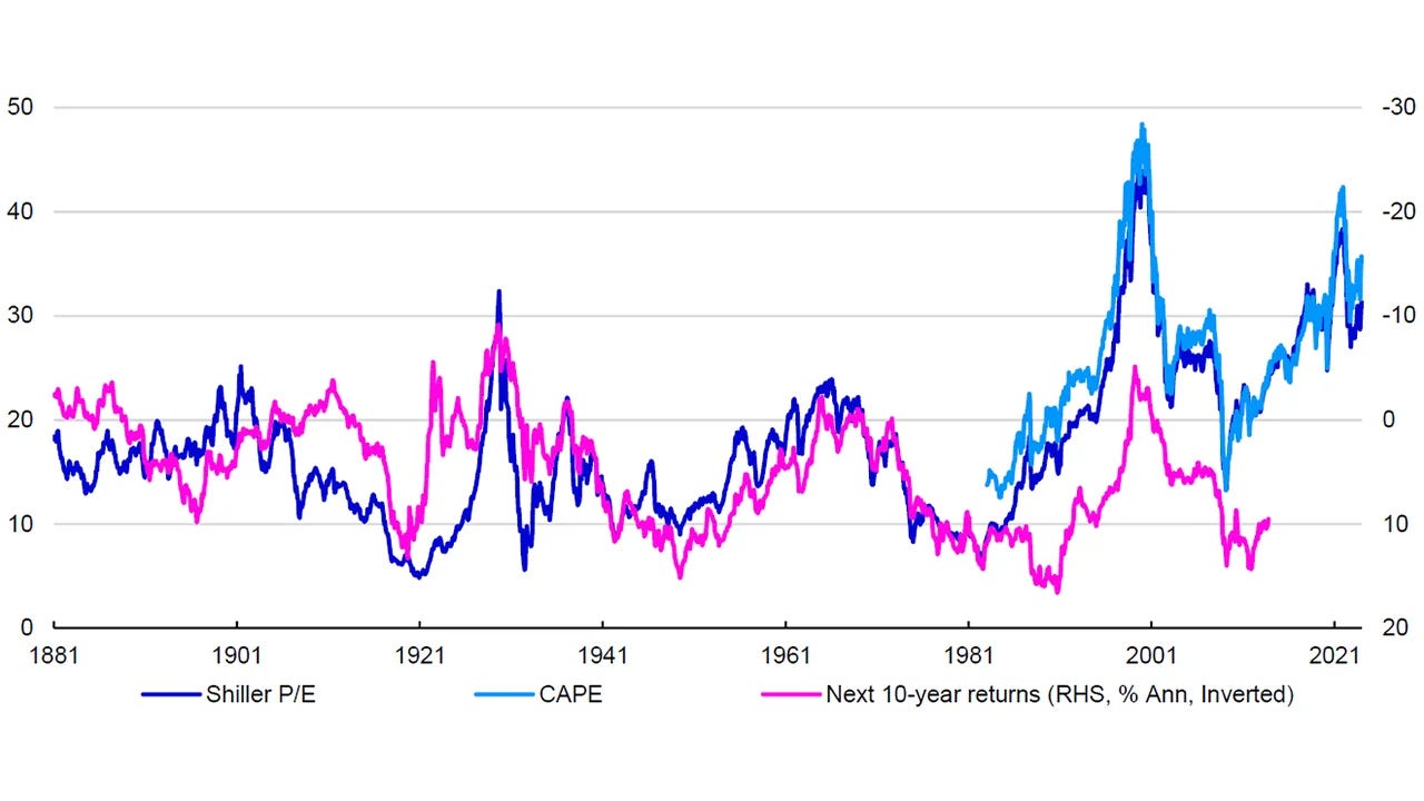
(Source: Invesco – LSEG Datastream, Robert Shiller, Invesco Global Market Strategy Office)

The challenge is defining this rigorously – in complex systems, propensities are not as clear-cut as a coin’s symmetry. Still, the propensity view reminds us there may be causal structures that bias probabilities (e.g. interest rates and earnings growth creating a predisposition for certain returns).

C) Subjective (Bayesian) Interpretation:

Probability as a measure of belief or confidence – essentially, a subjective degree of certainty.

In this view, “probability” lives in our minds (or models), not necessarily in the external world.

Saying “I estimate a 40% probability of a market correction in the next six months” is expressing a personal (or expert’s or model’s) degree of belief, given the information available.

This interpretation is very relevant to the stock market because different investors have different information and beliefs. One investor might assign a 20% chance to a recession, another 50%, based on their own analysis – those are subjective probabilities. They can be updated with new data (Bayesian updating).

(On April 9, 2025, betting markets were pricing in a less than 50% chance of a recession in 2025)

Subjective probabilities are coherent as long as one’s beliefs obey the usual probability axioms (and in theory, can be revealed by betting preferences – e.g. “I’d give 2-to-1 odds the market will be up this time next year” corresponds to a subjective 67% probability).

A classic illustration is that once a coin is flipped and covered, a person might say “there’s a 50% probability it’s heads” – even though physically it’s already determined. That 50% reflects their uncertainty, not the coin’s. Likewise, an investor might say “there’s a 50% chance of a bear market next year” – after the fact, the outcome will either happen or not (0% or 100% in hindsight), but beforehand that probability quantifies their uncertainty.

D) Bringing Them All Together …

So, how do these perspectives help us with a complex system like the stock market? Each offers a different lens:

• The frequentist approach encourages us to look at base rates and historical frequencies. For example, what percent of rolling 10-year periods in history had returns below inflation? (Answer: historically, only a small minority of 10-year periods have delivered negative real returns for U.S. stocks, but they do happen – e.g. late 1960s to late 1970s). What is the frequency of 50% drawdowns? How often has the market failed to recover to a new high for 10+ years? Using large samples of history or cross-sections of markets (like looking at other countries’ stock histories) gives a sense of the range of possibilities. This is critical for avoiding rosy predictions. A base-rate thinker might note, for instance, that historically the median annual return is a bit different from the mean – the distribution is skewed by big outliers. Frequentist analysis provides those reference points. But a limitation is that the market’s underlying conditions can change – the past frequency is not a guarantee. It’s an average of different regimes. If the future regime is fundamentally different (say, lower growth or higher inflation environment), the past frequencies could mislead.

• The propensity perspective in markets might lead us to build causal models – for example, economic models that assign probabilities to outcomes based on inputs. Think of stress tests or simulations: given interest rates, earnings, etc., we might say “there is a 30% propensity of a 0%–5% return, 50% propensity of 5%–10%, and 20% of >10%” under certain conditions. Analysts do something like this when they create scenarios (bull/base/bear cases) and attach probabilities to them – they are effectively assuming the setup (valuation, growth rates, etc.) creates an inherent likelihood distribution. Another example: When quants use Monte Carlo simulations for retirement planning, they are treating future returns as draws from an assumed distribution (often based on historical data or some theory). That assumed distribution is a statement of propensities – e.g. “we assume stocks have an intrinsic ~8% mean return with X% standard deviation, therefore the probability of a 20%+ loss in any year is Y%,” etc. The propensity view is appealing because it ties into the idea that the market has fundamental drivers (earnings, cash flows, valuation multiple changes, impact of buybacks, population growth, level of innovation) that set baseline probabilities. However, it’s very hard to verify propensities in the real world – you can’t rerun history to see how often 2025 “would” result in a 5% return. So we might have to rely on base rates and subjective judgment.

• The subjective (Bayesian) view is practically unavoidable in market forecasting. It acknowledges that we’re dealing with one incredibly complex sequence of events (the global economy/market over time), not a controlled repeatable experiment. Thus, any probability we assign to, say, “continuing 9.8% returns” is ultimately a subjective call – an informed guess. We update those guesses as conditions change. For instance, an investor might start 2023 believing there’s a 80% chance the bull market will continue; if a banking crisis hits, they might revise down that probability dramatically. This perspective is very useful when communicating uncertainty – e.g. one could say “I’m 60% confident that the next decade will see below-average market returns,” encapsulating their interpretation of data and intuition. It also allows incorporating personal or expert insight that might not be in the raw historical numbers (maybe you believe we’re in uncharted territory, so you weigh recent events more, etc.). The downside is that subjective probabilities can be biased or inconsistent – two people with the same info might have wildly different probabilities for the same event. That’s why Bayesian methods emphasize updating and coherence (and why things like prediction markets exist – to aggregate many individuals’ subjective probabilities into one consensus odds).

In academic literature, all three interpretations are discussed. Frequentist stats traditionally dominated fields like finance (e.g. calculating the probability of loss by looking at historical data). Bayesian approaches have gained traction in economics and investing for modeling uncertainty and updating beliefs. The propensity idea is more common in fields like physics, but in finance one could argue concepts like “true probability of default” or “underlying distribution of returns” hint at propensities, even if we can’t observe them directly.

To make this concrete, let’s apply each view briefly to the question of future stock returns:

• Frequentist/base-rate view: Historically, U.S. stocks averaged ~9.8% nominal. Out of (for example) 100 rolling 30-year periods in the past, 100% had positive real returns and, say, X% had 8%+ annualized returns​:

  

  (Source: Ben Carlson)

  Thus one might say the relative frequency of getting at least (for example) 5% real over 30 years was extremely high in the past. A base-rate analyst would start with that as a baseline, but also note the variance and that some periods did much better than others. They might also look at other countries’ 30-year stock returns to get a broader frequentist distribution – perhaps finding that while the U.S. never had a 30-year losing streak, a few other countries did due to catastrophes (which the U.S. avoided). So purely on frequency, one might say: if the future is like a random draw from the history of global markets, there is a small but non-zero chance of much worse outcomes, and also some chance of better-than-average outcomes – with a big middle probability around something mid-to-high single digits real return.

• Propensity/structural view: One might argue that the U.S. stock market has certain structural propensities – for example, an economic growth engine coupled with inflation over time gives a bias toward positive nominal earnings growth, and thus a propensity for positive nominal returns in the long run. There’s also a case that human innovation and productivity have an inherent upward drift, giving stocks a long-term propensity to rise (often summarized as “bet on human progress”). However, propensities can shift if structural factors shift (something we might be observing in real time in the US right now).

• Subjective view: Ultimately, each investor has to synthesize the data and their intuition into a personal probability distribution for future returns. For example, you might read all this historical data (frequentist) and the current indicators (propensity models) and conclude, say, “I believe there is roughly a 50% chance that returns will be significantly lower than 9.8% in the future, perhaps around 5%, a 30% chance they’ll be in a similar range as history (~8-10%), and maybe a 20% chance they’ll surprise on the upside.” Those numbers reflect your subjective belief given the uncertainty. They could be very different for someone else – e.g. a super-optimist might put a higher probability on continuation of historical performance (maybe they believe innovation or AI will boost growth, etc., and assign a 70% chance that stocks keep up a high return). Subjective probabilities are what we actually act on – whether explicitly or implicitly. Every time an investor chooses an asset allocation, they are implicitly expressing beliefs about the probability distribution of future returns (even if they just assume the past is prologue, that’s a belief).

No single interpretation is “right” – they complement each other. This may be the most important sentence in this entire blog. So let me repeat it:

A wise approach to market uncertainty might be: use frequentist base rates as a sanity check, incorporate structural/causal reasoning to adjust for how the future might differ from the past, and then form a subjective probability outlook that you update as new information comes in.

For example, academically, behavioral finance research shows that people often misestimate probabilities – they might overweight recent events (recency bias) or ignore base rates (base rate neglect). By knowing the historical stats (frequency) you guard against recency bias; by understanding propensity (causal factors), you guard against naive extrapolation of the past; and by refining subjective beliefs, you ideally avoid overconfidence.

So, when asking “will the 9.8% return likely continue?”, we’re essentially dealing with a probability judgment that should consider all these angles. Historically (frequency-wise), such high returns persisting was not unusual for the U.S., but structural factors and subjective assessments today might point to a more tempered expectation. This is where insights from experts on prediction and complex systems become relevant.

Part 3: The Limits of Prediction in a Complex Adaptive System (Lessons from Mauboussin and Others)

Financial markets are notoriously hard to forecast with precision. This section draws on the ideas of Michael Mauboussin and other thought leaders who have studied why prediction is limited in complex systems like the stock market, and how using base rates and humility can improve our approach.

Markets as Complex Adaptive Systems:

Michael Mauboussin describes the stock market as a textbook complex adaptive system​.

What does that mean?

Such a system consists of many interacting agents (in markets: millions of investors, traders, institutions) each making decisions and adapting to others. These interactions lead to emergent phenomena – the overall market behavior isn’t simply the sum of individual parts, but something richer and often unpredictable.

“Emergence disguises cause and effect,” Mauboussin explains – you can’t easily pinpoint a single cause for a market move because it emerges from countless interactions.

It’s akin to an ant colony: each ant follows simple rules, but the colony collectively exhibits complex behavior that no single ant understands.

Likewise, each investor might be reacting to news or incentives, but the overall market can do things (bubbles, panics, regime shifts) that are very hard to trace to one factor and even harder to predict in advance.

One key property of complex adaptive systems is non-linearity. Small inputs can lead to big outputs and vice versa, in non-proportional ways.

Think of a sandpile: adding one grain might do nothing, but adding one more grain at the right spot can trigger an avalanche. Financial markets have a similar property.

Because of this, prediction is extremely difficult. Mauboussin notes that in a complex system, “we don’t really know what’s going on” beneath the surface​ – we see outcomes but the causal chain is obscured by complexity.

First-order, linear thinking (“if A happens, then B will happen in the market”) often fails. For instance, one might think “rising inflation will cause stocks to drop”, which sounds logical in isolation (A causes B). But in reality, the market’s reaction includes second-order effects (How do people think others will react? What if investors expected the inflation already? What is the Fed’s counter-move?).

Often, the obvious cause-effect narratives break down.

“The stock market is a complex adaptive system in which linear thinking – A causes B and B causes C – isn’t sufficient”​ - Peter Lazaroff

Many “surefire” predictions (like “if candidate X wins, the market will crash”) have proven wrong because they were too linear, ignoring the adaptive, self-correcting nature of markets.

Another limit to prediction comes from the reflexivity of markets – participants’ expectations influence reality. If everyone expects 9.8% returns will continue, they may bid prices up (or take on leverage) in ways that actually reduce future returns or increase risk. This feedback makes forecasting a moving target.

The Base Rate and Outside View

In light of these challenges, experts like Mauboussin and Nobel laureate Daniel Kahneman suggest using the “Outside View” – essentially, start with base rates (historical or reference class data) rather than trying to predict from scratch using the “Inside View” of your specific situation.

Kahneman found that when people predict without outside data, they fall prey to the planning fallacy and overconfidence, envisioning rosy scenarios and ignoring how long things usually take or how often projects fail. The same applies to investors and economists making forecasts.

Mauboussin is a huge proponent of base rates in investing. He calls base-rate analysis a “wildly underutilized framework” for making forecasts.

What does this mean? Instead of saying “I think this time the market will do X because of Y reason,” first ask: what happened in all the other comparable times? For example, if we’re concerned whether the next decade’s returns might be subpar because stocks are at high valuations, we should gather data on all past instances of high valuation and see what happened subsequently.

That’s using the base rate of outcomes from a reference class.

The Limits of Expert Predictions

Even with good data, predicting complex systems has a poor track record. Philip Tetlock’s famous 20-year study on expert forecasts in politics and economics found that most experts barely beat random chance when predicting long-term outcomes​.

In his book Expert Political Judgment, Tetlock reported that the average expert was only slightly more accurate than “a dart-throwing chimpanzee” at forecasting future.

Many “experts” would have been better off simply guessing or extrapolating basic trends than following their detailed analysis, which often led them astray​.

One humorous finding: the more famous and frequently quoted an expert was, often the less accurate their predictions (possibly due to overconfidence or sticking to bold narratives)​.

This doesn’t mean we throw up our hands entirely – but it urges humility.

Financial markets amplify this difficulty because if any expert were consistently right, the market would adapt to price it in. Markets are somewhat efficient in that obvious edges get competed away. As a result, forecast errors are common. Mauboussin often cites the idea of the “Paradox of Skill”: as investors collectively get more educated and skilled, it doesn’t necessarily mean forecasts get better – instead, it means the competition is tougher and outcomes depend even more on luck.

When everyone is highly skilled, their predictions cluster and cancel out, and luck (randomness) plays a larger role in who comes out ahead​. This paradox could explain why, for example, most active managers underperform indices – not because they’re all incompetent, but because they’re all skilled and thus it’s hard to beat each other, and luck ends up dictating results.

Part 4: Conclusion

So what do Mauboussin and others recommend, given these prediction limits?

• Embrace uncertainty: Instead of single-point forecasts (“the market will return 10% next year”), think in scenarios and probabilities. Acknowledge a range of outcomes. Mauboussin suggests assigning probabilities and thinking in terms of expected value rather than precise predictions​. This aligns with a Bayesian mindset – continually update the probabilities as new data arrives.

• Use base rates (outside view) first, then layer in case-specific insight. If your specific prediction is way outside the historical distribution, you better have an extremely strong reason – otherwise, you’re likely overconfident or misinformed. For instance, if someone predicts “stocks will return 15% every year for the next decade,” the outside view says that would be an extreme outcome (better than nearly any past decade except the 1990s). Not impossible, but very optimistic against base rates. Thus one should treat such a prediction with skepticism.

• Focus on process, not point estimates: Because forecasting is hard, a good process (stock selection, valuation frameworks, portfolio construction) is more reliable than any one prediction. Mauboussin often highlights process over outcome – a sound strategy acknowledges uncertainty (e.g. holding a reasonably diversified portfolio because you might be wrong in your predictions).

• Recognize the limits of knowledge: As an investor, it’s useful to know what is knowable and what is not. We can be pretty confident about some base-rate things (like over 20-year spans, historically stocks have beaten cash the vast majority of the time​). But we should admit we cannot reliably call the exact return of the S&P next year or the precise timing of a crash. This is why many recommend a long-term horizon – over long periods, the noise of year-to-year volatility averages out, and things like economic growth and valuation mean-reversion tend to drive results (hence long-term outcomes are a bit more predictable in range than short-term outcomes). As Mauboussin and others say, the probability of losing money in stocks drops as your time horizon extends​ – so while we can’t predict short-term performance, we can tilt odds in our favor by lengthening the game.

• Beware of overfitting and false precision: Complex systems can produce patterns that are just noise. Numerous trading strategies that “would have worked” on past data fail in real time because they were just chance patterns (like finding shapes in clouds). Simpler, robust models often win out over highly complex predictive models that can break with regime changes. This echoes Nate Silver’s point in The Signal and the Noise – distinguishing real signals from noise in financial data is extremely challenging, but important!

• Learn from errors: Philip Tetlock’s later research on “superforecasters” found that some people can forecast better by constantly updating their views, mitigating biases, and learning from mistakes. They use practices like updating in increments as new info comes (Bayesian updating), looking at base rates, and breaking problems into components. Investors can try to do the same: if new evidence suggests a change (e.g. a structural shift in inflation regime), incorporate it rather than clinging to a prior prediction.

In summary, the experts teach us that confidence in long-term averages continuing should be tempered with an understanding of uncertainty and variability. Yes, use the historical 9.8% as a baseline, but don’t treat it as a law of nature. The stock market is a complex, adaptive, non-linear system – outcomes will sometimes stray far from averages, and our ability to foresee those deviations is limited. The prudent approach is to prepare for a range of outcomes and use probabilistic thinking.

We should also recognize that some aspects of future returns are easier to predict than others: for example, starting dividend yields and valuations give some information about the probable range of long-term returns (not precise, but they set boundaries – e.g. starting at a 2% dividend yield and moderate growth, it’s unlikely to get 15% annualized real returns for 20 years; likewise, starting at low valuations, it’s unlikely to get zero returns for 30 years).

But shocks, cycles, and investor behavior can dominate shorter periods.